1.3 A Discrete Probability Toolbox ​

Why probability in cryptography? Because “secure” is a claim about what an attacker can do, and the precise version of that claim is a bound on how often she succeeds: every definition we will use (perfect secrecy, pseudorandomness, unforgeability) bounds the chance of some bad event, such as the attacker guessing the key. This section collects the tools the rest of the tutorial needs: distributions, events, the union bound, random variables, independence, one lemma about XOR, and the birthday paradox.

Throughout, U is a finite set, most often U={0,1}n, the set of all n-bit strings.

1.3.1 Probability distributions ​

Think of a probability distribution as a set of weights, one for each outcome. Each weight is between 0 and 1, and together they add up to 1. A fair die gives each face weight 1/6; a loaded die gives one face more. Formally:

Definition (probability distribution)

A probability distribution P over a finite set U is a function P:U→[0,1] such that

∑x∈UP(x)=1.

Two extremes matter:

  • Uniform distribution: P(x)=1/|U| for every x∈U.
  • Point distribution at x0: P(x0)=1 and P(x)=0 for all x≠x0.

Concretely, for U={0,1}3 a distribution is exactly the vector

(P(000),P(001),P(010),…,P(111))∈[0,1]8

whose entries sum to 1. The uniform distribution on {0,1}3 assigns 1/8 to every entry; the point distribution at 101 is (0,0,0,0,0,1,0,0).

1.3.2 Events and the union bound ​

An event is a yes/no question about the outcome. “The last two bits are 11” selects some outcomes and excludes the rest; its probability is the total weight of the selected outcomes. Formally, for a subset A⊆U, define

Prx←P[A]:=∑x∈AP(x),

and call A an event. Necessarily Pr[U]=1.

Example: on U={0,1}8 with the uniform distribution, the event

A={x∈U:the last two bits of x are 11}

has probability 1/4 (a quarter of all strings end in 11).

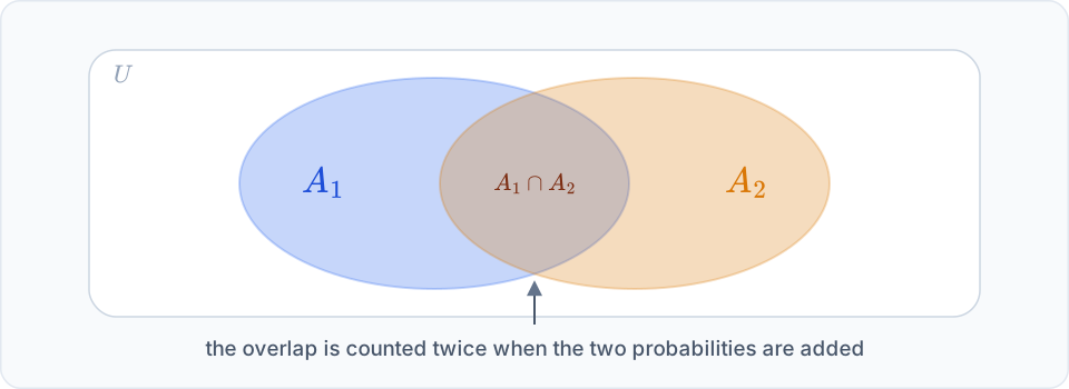
Two overlapping events A1 and A2 inside a universe; their overlap is counted twice when the two probabilities are added.

If either of two bad events would sink an experiment, the chance that at least one occurs is no larger than the sum of the two chances, because that sum counts the overlap twice. The one inequality you will use in every security proof:

Theorem (union bound)

For events A1 and A2,

Pr[A1∨A2]≤Pr[A1]+Pr[A2].

The proof is one line: summing over A1∪A2 counts each outcome in the overlap once, while Pr[A1]+Pr[A2] counts it twice. Induction extends the bound to finitely many events. In cryptography its work is always the same: “the attack fails only if one of the bad events A1,…,Aq happens; each has probability ≤ϵ; so the whole experiment fails with probability ≤qϵ.” Controlling a union of many small events is the standard move in a reduction proof.

Example: on U={0,1}n uniform, let A1 be “the last two bits are 11” and A2 be “the first two bits are 11.” Each has probability 1/4, so

Pr[A1∨A2]≤14+14=12.

(Here the true value is 7/16: the bound costs almost nothing and the slack is fine for proofs.)

1.3.3 Random variables ​

Think of a random variable as a numerical label attached to each outcome. Toss two coins and let X be the number of heads; then Pr[X=1] is the total probability of the outcomes with exactly one head. Formally:

Definition (random variable)

A random variable X (over U, taking values in V) is a function X:U→V.

Given a distribution on U, X induces a distribution on V: the probability that X outputs v is the probability of drawing an outcome x with X(x)=v.

Pr[X=v]:=Pr[X−1(v)]=∑x:X(x)=vP(x).

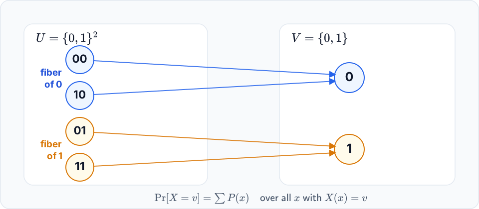
Example: X:{0,1}n→{0,1} defined by X(y)=lsb(y), the last bit. Under the uniform distribution on {0,1}n, exactly half the strings end in 0 and half in 1, so

Pr[X=0]=Pr[X=1]=12.
Four two-bit strings split into two fibers by their least significant bit and mapped to the values 0 and 1.

The mental picture: U is the sample space with its distribution P; X groups outcomes by the value they map to, and the probability that X=v is the total weight of the group for v (its fiber).

Quiz: Let r be uniform on {0,1}2={00,01,10,11} and define X to be the number of 1-bits of r. Find Pr[X=2].

X=2 happens only for r=11, so Pr[X=2]=Pr[r=11]=1/4. Likewise Pr[X=1]=1/2 and Pr[X=0]=1/4: X’s distribution on V={0,1,2} is not uniform even though r is. A random variable reshapes the distribution it inherits, so “uniform on U” does not imply “uniform on V.”

1.3.4 The uniform random variable and sampling notation ​

To say “we draw an element of U uniformly at random” we write

r←RU,

meaning: r is the uniform random variable on U, i.e. the random variable satisfying, for all a∈U,

Pr[r=a]=1|U|.

Formally, r is the identity map on U equipped with the uniform distribution. This notation will do heavy lifting later: k←RK for picking a key, c←E(k,m) for computing a ciphertext, and adversaries sampled like everything else.

1.3.5 Independence ​

Two events are independent when learning that one happened does not change the chance of the other. For random variables, independence means that no event about X tells us anything about Y. Formally:

Definition (independence)

Events A,B are independent if

Pr[A∧B]=Pr[A]⋅Pr[B].

Random variables X,Y (taking values in V) are independent if for all a,b∈V,

Pr[X=a∧Y=b]=Pr[X=a]⋅Pr[Y=b].

Example: r uniform on {0,1}2; X=lsb(r), Y=msb(r). Then

Pr[X=0∧Y=0]=Pr[r=00]=14=12⋅12=Pr[X=0]Pr[Y=0],

and the same check works for the other three pairs, so X and Y are independent. Independence is not a default. Two functions of the same uniform variable can be perfectly anti-correlated (lsb(r) and lsb(r)⊕1 always differ), so in proofs it must be either checked or assumed, and this tutorial will put “independent” in a hypothesis more than once. The crucial instance arrives with XOR.

1.3.6 Randomized algorithms ​

A randomized algorithm is allowed to toss fresh coins while it runs, so two runs on the same input may differ. Formally, a deterministic algorithm takes an input m and produces y←A(m). A randomized algorithm also reads fresh random coins:

y←A(m;r),r←R{0,1}n,

and its output is a random variable. Encryption is the familiar example, A(m;k)=E(k,m), in which the key is the random coins. From Chapter 2 onward, “attacker” will always mean a randomized algorithm, and security definitions quantify over the randomness of both the scheme and the adversary. This is why all of the probability above is needed: a claim that “the attacker wins with probability at most 2−100” has no meaning until you say over which coins.

A deterministic algorithm A takes m and returns the same y every run; a randomized algorithm also reads fresh coins r from the set of n-bit strings, so its output is itself a random variable.

1.3.7 XOR and the masking lemma ​

The bitwise XOR of two strings in {0,1}n is their bit-by-bit addition mod 2:

0110111⊕10110101101101

For every fixed s, the map x↦x⊕s is a bijection of {0,1}n onto itself, and its own inverse. That is what makes XOR a mask: XOR with a fresh uniform string leaves no trace of the original value. The single most useful lemma in the first half of this tutorial:

Theorem (masking lemma)

Let Y be any random variable over {0,1}n, let X be uniformly distributed on {0,1}n, and let X and Y be independent. Then

Z:=Y⊕X

is uniform on {0,1}n, whatever Y is.

Proof for n bits: fix any a∈{0,1}n. Partition the event “Z=a” according to the value y that Y took:

Pr[Z=a]=∑y∈{0,1}nPr[Y=y∧X=a⊕y]=∑yPr[Y=y]⋅Pr[X=a⊕y],

where the second equality is independence. But X is uniform, so Pr[X=a⊕y]=2−n for every y:

Pr[Z=a]=∑yPr[Y=y]⋅2−n=2−n∑yPr[Y=y]=2−n⋅1=2−n.

Since a was arbitrary, Z is uniform. ∎

Read the theorem as a security statement: with Y a message and X a fresh uniform key, the ciphertext Y⊕X is uniform, so it is independent of the message, and an eavesdropper sees a string indistinguishable from coin flips. That is the one-time pad, and the lemma is nearly its whole proof; the rest is making “sees nothing” precise. Keep X fixed and reuse it for many messages, and the lemma no longer applies, which is the one-time-pad-versus-Vigenère lesson of Section 1.2 in one line of algebra.

1.3.8 The birthday paradox ​

The birthday phenomenon is a statement about pairs rather than samples: the chance of a collision grows roughly like n2/|U|, and the theorem makes the threshold precise:

Theorem (birthday bound)

Let r1,…,rn be independent, identically distributed random variables, each uniform on a finite set U. When

n≈1.2⋅|U|1/2,

the probability that some pair collides, Pr[∃i≠j:ri=rj], exceeds 12.

Derivation: work with the complement. “No collision” means r2∉{r1}, r3∉{r1,r2}, and so on, so

Pr[no collision]=1⋅(1−1|U|)⋅(1−2|U|)⋯(1−n−1|U|).

Each factor satisfies 1−x≤e−x, so the product is at most

exp(−1+2+⋯+(n−1)|U|)=exp(−n(n−1)2|U|),

and therefore

Pr[collision]≥1−e−n(n−1)/(2|U|),

which is the familiar 1−e−n2/(2|U|) with n−1 replaced by n. At n=1.2|U|1/2 the exponent is 1.44/2=0.72, and 1−e−0.72≈0.51>12. ∎

The proof assumes a uniform distribution; for non-uniform distributions collisions are only more likely, so the guarantee still holds.

The name comes from birthdays: with U={1,…,365} the threshold is 1.2365≈23, so 23 people in a room are enough to make a shared birthday more likely than not. The reason is that n people contain (n2)≈n2/2 pairs, and it is the pairs, not the people, that collide. Collision risk grows like n2/|U|, which means a space of size |U| gives out after about |U| samples.
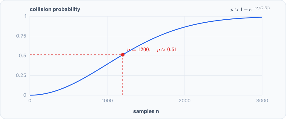
Collision probability rising with the number of samples for a space of size one million, crossing one half near 1200 samples.

A worked table for |U|=106 gives:

n (samples)collision probability ≈1−e−n2/2⋅10−6
1,0000.39
1,2000.51
1,6000.73
2,1000.89

With U={0,1}128, about 264 samples suffice to produce a collision, so a 128-bit space gives out after about 264 samples; the cryptographic use of this bound arrives in Chapter 5.

With the notation in place, Chapter 2 asks what is a secure cipher, and answers it exactly, once: the one-time pad.

Powered by VitePress